Cluster-based Penalty Scaling for Robust Pose Graph Optimization
- Supplementary material
This supplementary material is organized in two sections. In Section I we provide details on how group outliers are generated and present an in-depth analysis of the experimental results for group outliers. In Section II we perform parameter study on the effect of the penalty scaling for pro-odometry clusters.
I Effect of outliers’ structure
Originated from Sunderharf’s work [4], research on outlier mitigation [3, 1, 2] has commonly injected two types of outliers into clean datasets for performance validation: random outliers, where singular outliers are generated by randomly choosing a pose-pose pair and no inner structure among outliers are enforced111Note that inner structure can still form, since one randomly generated singular outlier can be consistent with some other randomly generated singular outliers. The emphasis here is that it is not enforced.; and group outliers, where a specific inner structure is enforced on the outliers so that within one group, all the edges are consistent with each other topologically. We also used the script from [4] to generate random singular outliers. However, the proposed group outlier generation scheme has three fundamental issues:
-
It produces all outliers in groups. This is equivalent of assuming all outliers during the whole trajectory are generated from perceptual aliasing instances that produce mutually-consistent outliers, ignoring random singular outliers entirely.
-
All groups have the same number of outliers. This is equivalent of specifying all the perceptual aliasing instances to span the same number of poses.
-
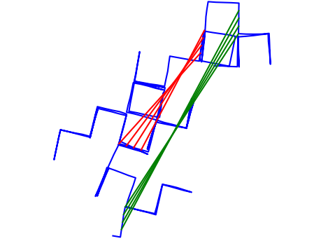
With each edge referred as , the poses of the edges in one group are in strict consequential order. So are the poses. An example is shown in Fig.0(a).
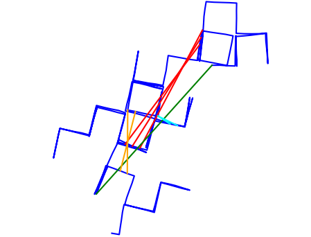
Based on our observations, these three conditions are rarely true in reality. Group outliers exist together with random singular outliers most of the time, and individual perceptual aliasing instances natually produce different number of mutually-consistent outliers. To improve and simulate perceptual aliasing in a more realistic way, we design a new scheme for group outliers generation, shown in Algorithm 1. Instead of constraining the number of loop closures in all groups to be one constant, our method produces a mixture of singular outliers and group outliers of different sizes. In addition, instead of strictly consequential edges, we randomly generate the pose-pose pair within a specific range and inject a noise level of pose. The differences between group outliers from [4] and our methods are illustrated in Fig. 1.
|
|
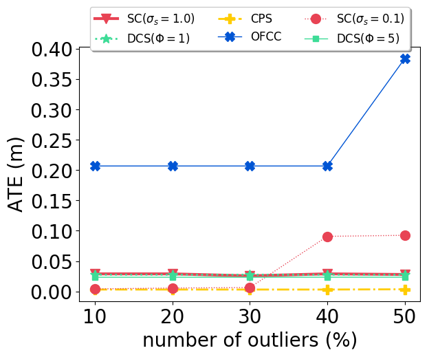
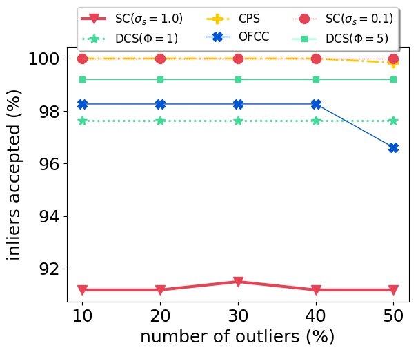
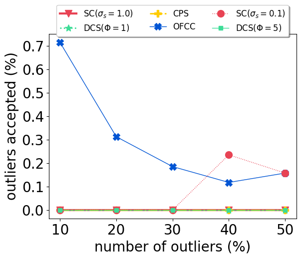
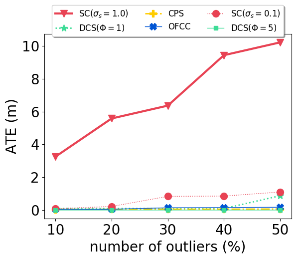
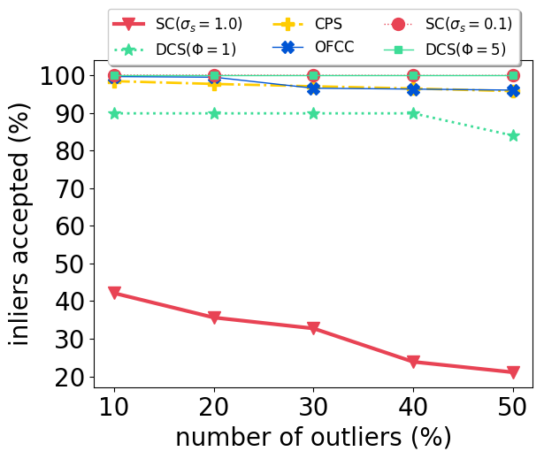
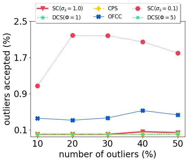
With our carefully designed group outlier generation schemes, we conduct experiments on datasets with 10%, 20%, 30%, 40%, 50% outliers. Experimental results on CSAIL are shown in Fig. 2. OFCC performed much worse than other methods by accepting more outliers. SC (), DCS and CPS had stable performance regardless of the number of outliers. And CPS achieved the lowest ATE by rejecting most outliers and also accepting most inliers. For DCS, different value didn’t affect the ATE significantly. SC () performed better than SC () when the number of outliers is low, but soon deteriorated by accepting more outliers as the number of outliers is higher than 30%.
|
|
|
|
|
|
|
|
|
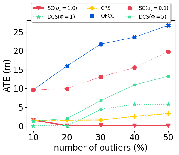
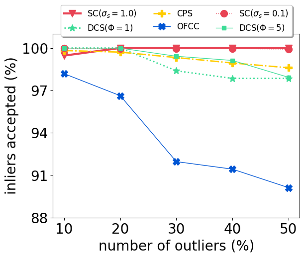
Experimental results on the Manhattan datasets are shown in Fig. 3. Both OFCC and SC () failed due to accepting outliers even at 10% outliers. And in doing so, OFCC rejected a lot more inliers then other methods. Both DCS () and DCS () performed reasonably when the number of outliers were low, but soon deteriorated as the number of outliers increased. SC () achived the lowest ATE on this configuration, rejecting all outliers while still accepting most of the inliers. CPS performed as well as SC () at low number of outliers, and its performance slowly deteriorated as the number of outliers increased. We note that this is the only configuration in our experimental setups that CPS performed slightly worse than another method, although we can still observe that it avoided accepting loop closures that would cause large global distortion: comparing its performance and DCS, both DCS () and DCS () accepted less outliers than CPS, but had much higher ATE.
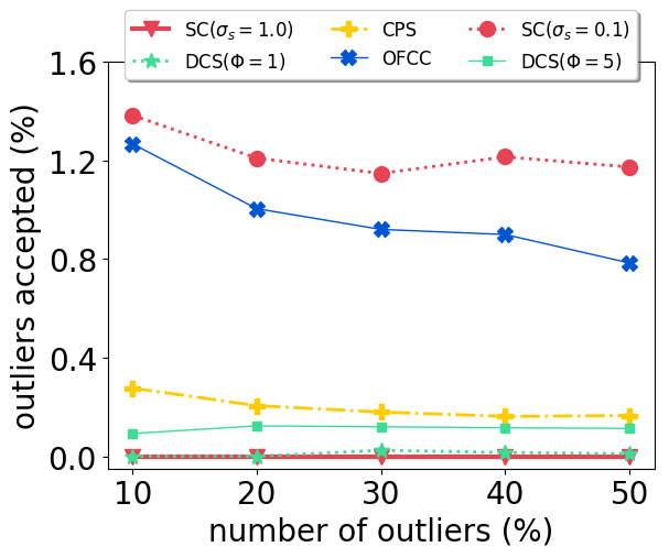
Experimental results for the Intel dataset are shown in Fig.4. SC () failed by rejecting too many inliers while SC() performed significantly better by making good compromise. DCS () performed well untill the number of outliers is at 50%, while DCS () is not affected. OFCC and CPS performed consistently well regardless of the number of outliers.
Comparing the experimental results presented here and those for random singular outliers, we note that the outliers’ structure affects the performance of state-of-the-art methods in various ways: OFCC performed significantly worse on CSAIL with group outliers than with random outliers. SC () performed significantly differently for the group outliers and random outliers on the CSAIL dataset, making parameter tuning even more difficult. Our proposed method not only performed better or comparable with other methods at their best parameters, but also exhibited similar behaviors for outliers with different structures. Its performance deteriorated gracefully as the number of outliers increased.
Ii Effect of Penalty Scaling on pro-odometry cluster
As explained in the paper, we treat the pro-odometry clusters differently by decreasing by a factor 10. Here we conduct an ablation study on this strategy to examine its usefulness. We refer to this parameter as here to differentiate it from the variance of the prior constraints for against-odometry clusters, which is set to 1.0 at all times.
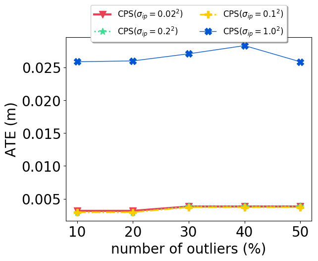
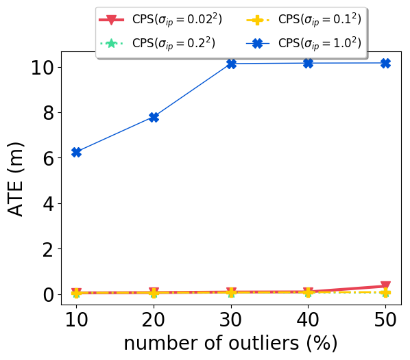
We vary the parameter value: , to examine its effect on performance. When , it is equivalent to disabling the scaling strategy for pro-odometry clusters since the same variance is used for against-odometry clusters. Experimental results on the CSAIL and Intel datasets are presented in Fig. 5. It is apparent that when the scaling strategy is disabled, the ATE significantly increases on both datasets, and the effect is much more severe for the Intel dataset, due to its noisy odometry. When the strategy is enabled and with varying parameter values, the ATE changes by a negligible amount, with the only exception being for the Intel dataset. For this configuration, the highest ATE is still below 1m. For the Bicocca dataset, the ATE increases from 1.102m to 2.905m when the scaling strategy is disabled, and reduced to 0.661m when , 0.605m when .
|
|
In summary, we can conclude that treating pro-odometry and against-odometry clusters differently with penalty scaling played a significant role in our method. And despite having one extra parameter for the pro-odometry clusters, the performance of our method is only minimally affected when a wide range of parameter values are used. It is significantly less sensitive to parameter tuning compared to other methods.
References
- [1] (2013) Robot Map Optimization using Dynamic Covariance Scaling. 2013 IEEE International Conference onRobotics and Automation (ICRA). Cited by: §I.
- [2] (2014) Selecting good measurements via relaxation: A convex approach for robust estimation over graphs. IEEE International Conference on Intelligent Robots and Systems, pp. 2667–2674. External Links: Document, ISBN 9781479969340, ISSN 21530866 Cited by: §I.
- [3] (2018) Modeling Perceptual Aliasing in SLAM via Discrete-Continuous Graphical Models. pp. 1–13. External Links: 1810.11692, Link Cited by: §I.
- [4] (2012) Switchable constraints for robust pose graph SLAM. IEEE International Conference on Intelligent Robots and Systems, pp. 1879–1884. External Links: Document, ISBN 9781467317375, ISSN 21530858 Cited by: 0(a), §I, §I.